Machine Learning Algorithms on Fake News Detection — With Comments

Part 1: Naïve Bayes Algorithm

Naïve Bayes is an algorithm that utilizes the Bayes Theorem in text classification.

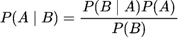
For a text-based data set, Naive Bayes computes the posterior probability for each class by multiplying the likelihood of each word (in the document) for that class and multiplying it by the class prior. The class with the highest posterior probability is chosen as the predicted label.

Code Implementation

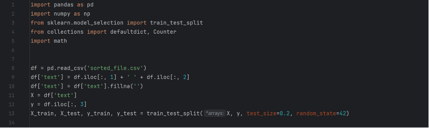
The first part consists of preparations, including importing libraries, loading the data set into a data frame, and splitting the data set. Important takeaways include 1) I used the .fillna() function to replace all blank and incorrectly formatted values in the second, or “text”, column, because I found the data set to be prone of errors 2) I reserved 20 percent of the dataset for testing, and 80 percent for training, and the random number ensures that the split is the same every time for reproducibility of results.

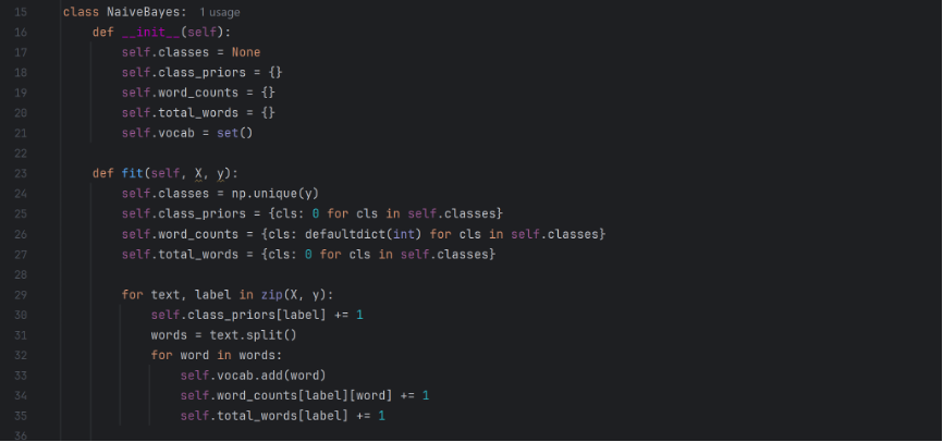
Subsequently I proceed with the Naïve Bayes classifier. I define a classifier class NaiveBayes, and create spaces to store the two classes (real and fake), the prior probability of each class, the frequency of each word for each class, the total number of words for each class, and the total vocabulary of the dataset. I them create the fit function to train the dataset. It first finds the labels (either real or fake), and them initializes the parameters mentioned above. Them it loops through each document, split the text into words, and increment on the respective parameters.

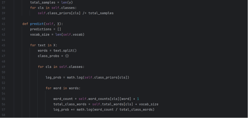
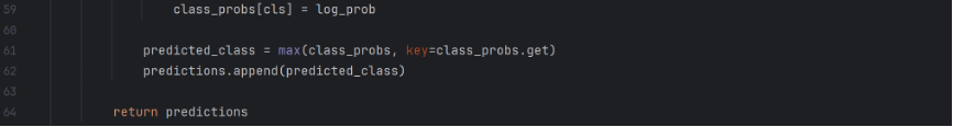
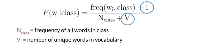
Now the class counts can be divided by the total number of samples to derive the probability. The predict function predicts the classification of new samples. Coming upon a particular text, the function browses through each word and, based on the prior probability derived from the previous training model, accumulates the results to chooses the class with a higher likelihood. Note that I incorporated Laplace smoothing in my calculations in order to deal with words that didn’t appear in the dataset and is new to the model.

Lastly, the function returns the list of predictions.

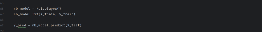
The training and testing data are now assigned to the respective functions.

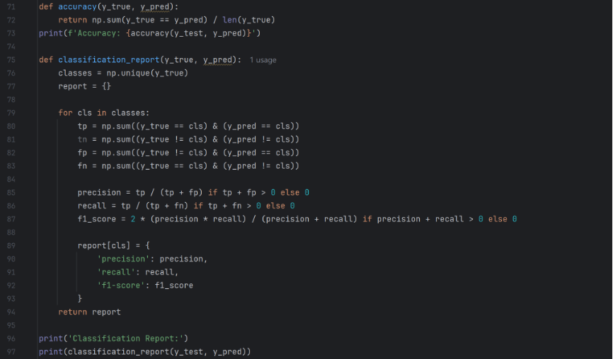
A report is now generated. It outputs first the overall accuracy, and then the precision, recall, and f1-score statistics for both classes. Here are the results.

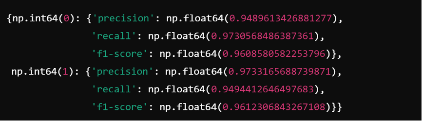
To begin with, the overall accuracy rates 96.1% percent, proving that the model is relatively reliable. Precision is the ratio of true positives to the total predicted positives for the class, recall is the ratio of true positives to the total actual positives, and the F1-score is the harmonic mean of precision and recall. The results with precision (97.33%) higher than recall (94.94%) for fake news (Class 1) and recall (97.31%) higher than precision (94.90%) suggests that my model is conservative for fake news. It is cautious in labeling something as fake, at the expense of allowing a slightly larger amount of fake news to be considered as real. This might mean that my model would be better suited in circumstances where it is more important for real news to be heard, and the harms of fake news are relatively subtle.

Improvement

In order to examine the shortcomings of my model I devised a new set of codes to output a misclassification report. The misclassification report identifies the number of misclassified instances, the most common words in misclassified text samples, and the average length of misclassified text.

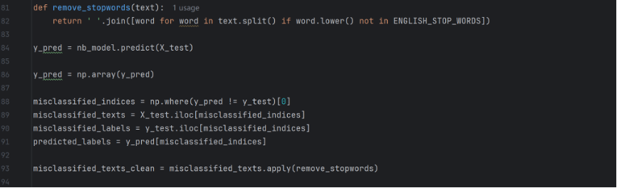
For the same model I now have it produce a misclassification report instead of accuracy report. I first write a function remove_stopwords to remove stop words when analyzing, because if not then the most common words in the mistaken text would turn out to be words like “the” and “to”, which doesn’t help the analysis. Then identify the misclassified instances and apply the function.

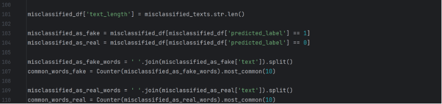
This counts the word frequency in misclassified instances.

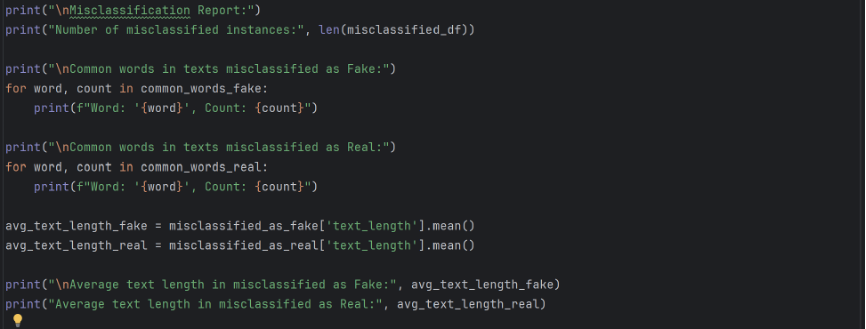
Here are the results to the misclassification report.

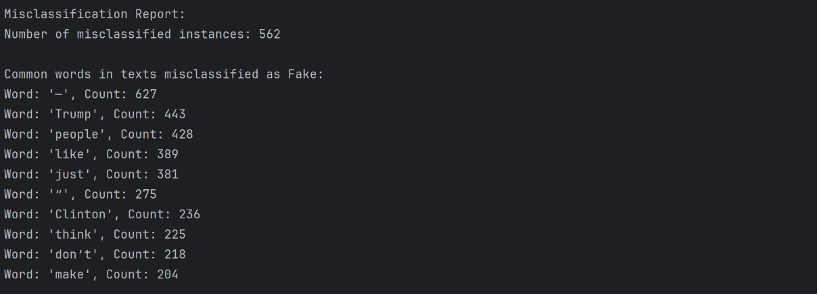
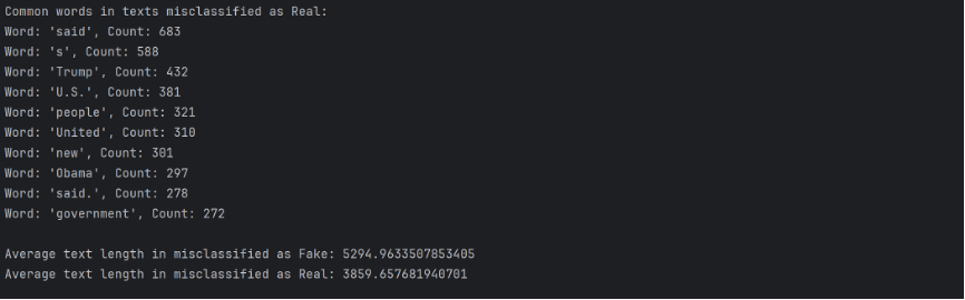
Key takeaways: 1) Many words related to politics, such as “Trump”, “Clinton”, “United”, show up frequently in misclassified texts, implying that the model may have a hard time identifying politics related pieces of news. 2) The average length of text misclassified as fake greatly exceeds the average length of text misclassified as real, implying that the model might have falsely label many pieces of news as fake because their sheer length guaranteed that they are more likely to have shared more words with fake news texts.

Part 2: Logistic Regression

The logistic regression model first computes a linear combination of the input features and the model’s weights, plus a bias term:

z is the linear combination, x_1 to x_n are the inputs, beta_1 to beta_n are the weights, and beta_0 is the bias. The linear combination is them translated into a possibility value with the sigmoid function:

It maps z to a possibility between 0 and 1. The piece of news is considered fake if y is greater than 0.5, and real if y is less than 0.5. The model is trained through gradient descent to minimized binary cross-entropy loss, which is expressed with the form:

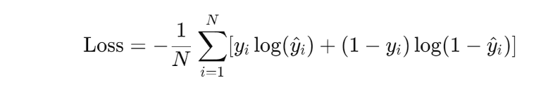
Where y^_i is the predicted label, y_i is the true label, and N is the total number of samples.

Code Implementation

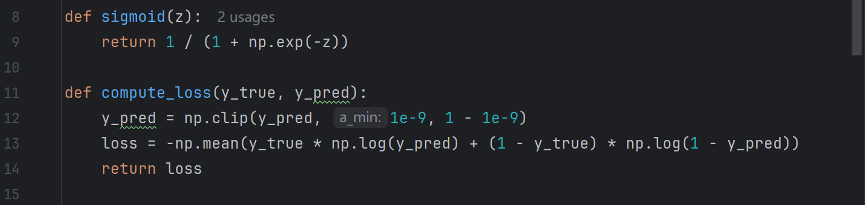
These two functions are defined to compute sigmoid function and binary cross-entropy loss. The np.clip function guarantees that the values wouldn’t be exactly 0 or 1, since calculating log(0) or log(1) would create problems for the program.

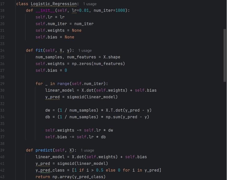
The function “init” initializes the model and defines learning rate, number of iterations, weight, and bias. “fit” then defines the training model and sets initial weight and bias to zero. The subsequent loop function is the core of logistic regression. “linear-model” is derived by multiplying the samples matrix with the weights and adding the bias, and then it undergoes the sigmoid function to be translated into a possibility. “dw” stands for the gradient of the loss function with respect to weight, and “db” stands for the gradient of the gradient of the loss function with respect to bias. These values reflect how much the weights and bias need to be changed. The values are then adjusted with regards to dw and db, and learning rate determines the size of the update. The “predict” function conducts the predictions, turning the possibilities into predictions of fake or real.

In order to feed the news texts into a linear combination, the texts need to be transformed into the TF-IDF format.

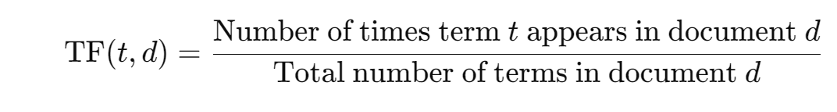
TF stands for Term Frequency, which reflects the frequency of a particular word in a particular text.

IDF stands for Inverse Document Frequency, which reflects the rarity of a particular word in the entire data set. N is the total number of texts and DF(t) is the number of texts that contains the word.

Each word in each document has a unique TF-IDF value, which reflects its importance of this word. A high TF-IDF score shows that the word is relatively important to a particular article and is also not commonly seen in all texts.
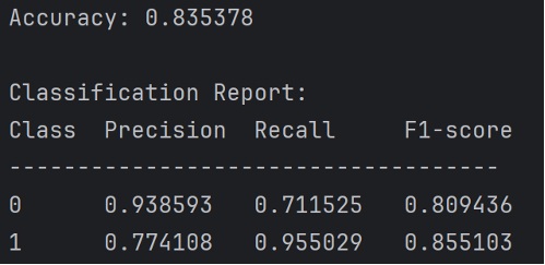
Here are the results of this model.

Improvements

In order to analyze the potential reasons for the precision-recall imbalance in the model, I devised several methods. Diagnostics of the model is based on the following aspects: class imbalance, confusion matrix, precision recall curve, feature importance, and threshold adjustment.

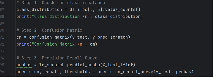
To begin with, a majority of a particular class of news might alter the precision and recall values of a logistic regression model. Secondly, reporting a confusion matrix can help better analyze the results. The precision-recall curve is meant to find an optimal balance between precision and recall, and therefore tweak the threshold to make it match the balance.

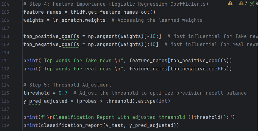
Feature importance examines the relative frequency of words in misclassified texts.

Conclusion

In this report I have conducted fake news detection with two algorithms, Naïve Bayes and Logistic Regression, and these models shows respectively their unique advantages and disadvantages. Furthermore developments could be focused on algorithms that can analyze consecutive phrases and texts instead of particular word frequencies, such as deep learning with neural networks.